The basics of Financial Wave Theory (FWT)
What is the Financial wave theory
The financial wave theory is an elaboration by CVC’s director Ahmed Farghaly on prior work made on economic cycles. It is based on the logic that after a certain period of time has passed people tend to repeat prior forgotten mistakes when confronted with a similar environment. This leads to measurable correlations on the price chart which can in turn lead to successful forecasts of the future. Usually, different players are involved in the marketplace today than the similar environment in the past being used to obtain the forecast of the future. This is due to the fact that the shortest cycle we use in FWT is the 18-year cyclical position. Such correlations with large cycles are much more pronounced considering that the players are different yet human nature remains the same hence similar actions can be expected. The theory is based on CVC’s nominal cyclic model which we put together back in 2016. The cyclic model is presented below
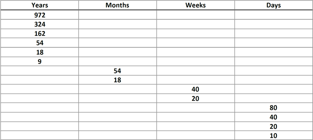
Our work here at CVC consists of finding our current position within the longer-term waves presented above and obtaining projection lines for the future course of prices for each wave. Recall from earlier that we are only interested in the cyclic positions of the 18-year wave and above (54 years, 162 years, 324 years, 972 years). Based on historical data, that we have at our disposal, we were able to depict the cyclical position of core nation-states going up to the 324-year cycle position. For the 972-year cycle, we can only guesstimate considering that we don’t have data to actually come up with an accurate phase of the cycle. Notice that all the cycles presented above are harmonically related (which J.M. Hurst has called the principle of harmonicity) i.e., the smaller cycle is related to the next larger cycle by a multiple of 2 or 3. Let us present what we mean by utilizing ideal waves in the following two images.
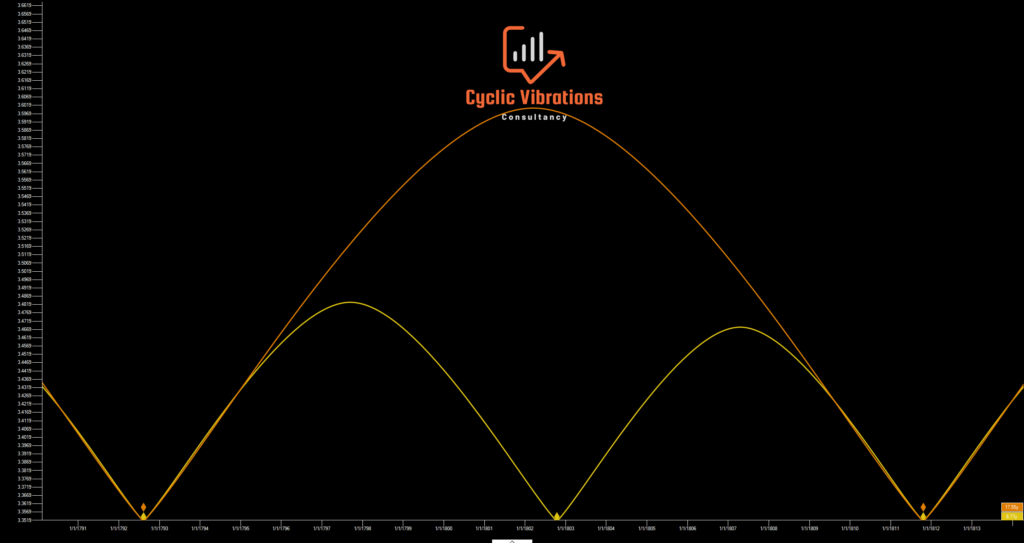
The presentation above presents an 18-year cycle on the S&P500. From a historical context, this was the first 18-year swing (Kuznets) within the second 162-year wave (Jared) within the 324-year cycle (Enoch). Notice how this 18-year wave subdivides into its second harmonic the nominal 9-year wave (Juglar). Notice that the amplitude (height of the cycle) in the 9-year wave is half that of the 18-year cycle (Hurst called this the principle of proportionality)
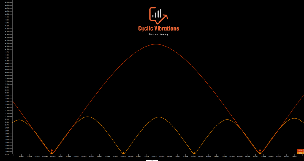
The chart above presents the preceding 54-year swing (Kondratieff) relative to where we stand today. Notice that both the principle of harmonicity and proportionality are evident in the chart above. The Kondratieff wave is subdivided into 3 Kuznets swings. Another cyclic principle worth noting is the principle of synchronicity which suggests that, whenever possible, the larger cycle troughs coincide with the troughs of all cycles that are smaller in length than the main cyclical low. This means that a low in the Kondratieff wave will always coincide with a low of the Kuznets, Juglar, Kitchen (54 month), and all smaller cycles at the same time. The opposite does not hold true, meaning that not every Kuznets cycle low will coincide with the larger Kondratieff low since the larger cycle contains three Kuznets swings. If you were to analyze the period of the two Juglar cycles presented in figure 2 you will realize that they are not exactly the same which brings us to our next principle in cyclic analysis known as the principle of variation. The principle of variation suggests that cycles exhibit variation in period (time length of the cycle) and amplitude. This means that the period and amplitude (price differential within the cycle) of two adjacent cycles of the same wave need not be identical yet will tend to be similar. The issue of variation is more pronounced when a larger sample size of cycles is examined. This is why cyclic analysis is best applied to a limited number of price bars to avoid the confusion that could arise due to the principle of variation. At CVC, we analyze the entire recorded history of prices when examining a specific index or commodity. The reason why we do so is to find our position within the larger cycles spoken off to get projections with high out-of-sample correlations. The more distant the analog used is from the present the higher the correlation. There is a logical reason and a technical reason behind the previous statement. The logical reason is: As humans, we have a tendency to draw historic parallels between the current environment and the past. This means that the more distant the analog is from the present day the higher the likelihood of current participants not drawing a parallel with that particular instance hence will be more correlated with the present and the future. The technical reason for the statement above is the higher similarity in trend (distant past and present) when utilizing the correct starting point. The concept of the trend will be considered in great detail in a future post. Another important cyclic principle we would like to discuss in this post is the principle of commonality. The principle of commonality suggests that all available financial instruments have many things in common. They all adhere to the same cyclic model and exhibit all of the other cyclic principles mentioned in this post. They also tend to experience major cyclic lows in unison or significantly close to each other in time. If we look at the long-term cycles on both the Dow Jones Industrial Average and CRB index we will notice that the cyclic lows do their best to coincide with one another. This argues that there is a single underlying force vibrating beneath all markets yet affects each of them in a slightly different manner. This is an idea we subscribe to here at CVC.
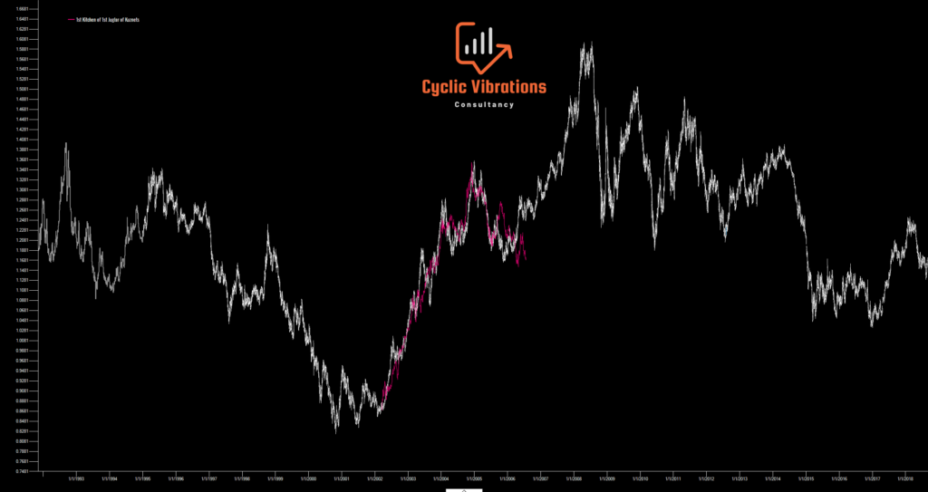
Figure 4 presents the kind of correlations that can be obtained utilizing the financial wave theory. The cycle being used was the first Kitchen within the first Juglar of the Kuznets swing on the EURUSD, a position we were under starting in 2002 and in 1985. The line in pink is from 1985 to 1989. We must remember that the principle of variation stops us from obtaining projections this accurate by overlaying the price with the same time scale. We mentioned that the period of the cycle of a given wave (54 month in this instance) can change slightly over time. To account for the principle of variation, we must alter the time scale of the similar cyclical circumstance (1985-1989) to arrive at an optimal forecast. In this particular example, we multiplied the time scale by 0.97!
Regards,
CVC research team