Our software’s forecast on the Euro against the US Dollar from April 2002 to July 2006.

Our introduction to the financial markets came through the foreign exchange market in 2008, following the price increase of the US Dollar as a result of the economic crisis. Everyone expected the price rise of the US Dollar to continue, as a result of an extreme sentiment typical near a significant price high. The volatility present during the economic crisis has, for the most part, subsided, except during the double-dip recession experienced in Europe from 2011 onward. In today’s article, we will present how our software forecasted the price movement after the Kuznets swing low in April 2002 into the following Kitchen cycle trough anticipated in July 2006 on the Euro against the US Dollar (The trough came several months earlier than the expectation based on the mean period of the Kitchen cycle).

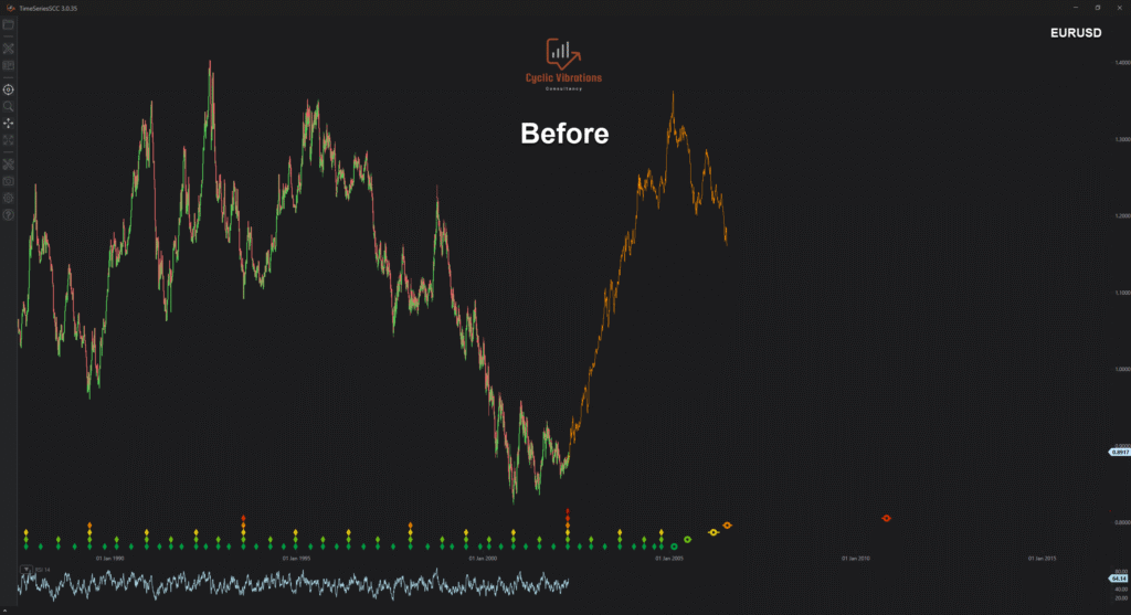
Figure 1 presents our expectations for the Euro against the US Dollar from April 2002 to July 2006. As visible from the diamonds on the bottom, we have most likely entered the early stages of the Kuznet’s swing, which would suggest a significant change in trend to the upside for the near, intermediate, and distant future. Our attempt here was to construct a price movement forecast for the first Kitchen cycle within the newly initiated Kuznets swing. We based the scale on the current average period of the Kitchen cycle. It is essential to note that this is a good starting point. Still, it will prove more fruitful to scale the projection based on the minor cycles of the Kitchen cycle, which we are attempting to forecast as soon as the opportunity presents itself. Let us now see how well this projection has forecasted the future price movements of the Euro against the US Dollar below.

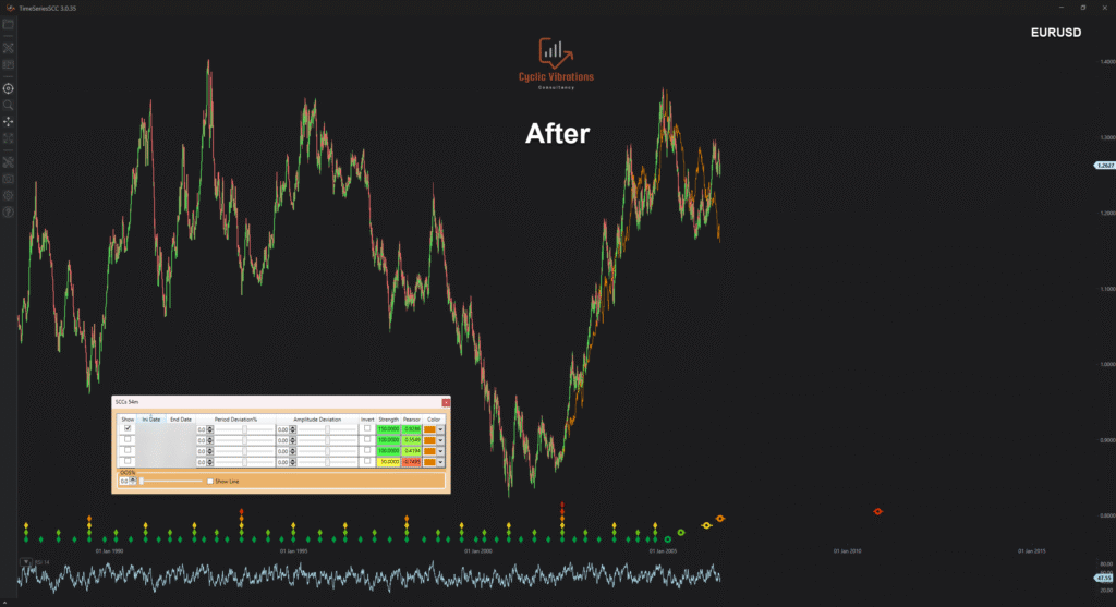
The correlation coefficient of our forecast with future prices was a whopping 0.9286! This is a forecast that lasted an entire Kitchen cycle without altering or changing the scale of the projection. If we had applied our methodology of scaling the projection based on the minor cycles, we would have approached a correlation coefficient of 0.96. This is the fifth example we present in our blog that resulted in a correlation coefficient of over 0.9. Don’t think that we will stop here; we will continue to present you with many more examples until you are convinced that nothing out there is being offered that comes even close to our proprietary methodology. It is essential to note that sometimes fundamental factors in either the analog or the current cycle can affect the correlation coefficient between them. That is why price movements in the analog that occurred due to one of the fundamental factors discussed in a later post should be expected to reduce the overall correlation coefficient with the current cyclical circumstance. When we state fundamental factors, we are not referring to the general fundamental environment that is similar between the SCC and the CCC. Instead, we are referring to fundamental factors that cause a disruption that the cycle theory cannot explain. Thankfully, the presence of such factors is usually rare, which does not diminish the overall value added by the application of the Economic Wave Theory, as presented in the current and prior articles posted on our blog. We currently hold a future projection for the Euro against the US Dollar that is free of fundamental factors, which should ideally lead to high correlation with the current cycle, provided it too is free of fundamental factors. We would guide you to our services page to book a consultation on this instrument if you wish. In the meantime, we will keep our fingers crossed!

Thank you for your time,

CVC research team